Posts with #MatLab

#MatLab

Public posts on X that use #MatLab.

Related hashtags

  1. MATLAB@MATLAB
    Transform your work by watching this video on how to use MATLAB. Get the ins and outs of designing and analyzing electrical systems with MATLAB's powerful toolboxes and functions. #MATLAB #ElectricalSystems #Simulation
    Download
    23526441K
  2. Jousef Murad@Jousefm2
    The #matlab code here at the source: Implementation of a vorticity-streamfunction method with a pseudo-spectral discretization + third-order Runge-Kutta for time integration.
    Download
    Computational Fluid Dynamics group @CFDonia
    Following many two-dimensional turbulence animations, it is time to share computer code! Implementation of a vorticity-streamfunction method with a pseudo-spectral discretization + third-order Runge-Kutta for time integration (our CFD class semester project). The @MATLAB code: M = 256; % number of points N = M; Lx = 2*pi; Ly = 2*pi; nu = 5e-4; % kinematic viscosity Sc = 0.7; % Schmidt number beta = 0; % meridional gradient of Coriolis parameter ar = 0.02; %random number amplitude b = 1; % mean scalar gradient CFLmax = 0.8; tend = 200; % end time x=linspace(0,Lx,M+1); x(end)=[]; dx = Lx/M; kx=[0:M/2 -M/2+1:-1]*2*pi/Lx; y=linspace(0,Ly,N+1); y(end)=[]; ky=[0:N/2 -N/2+1:-1]*2*pi/Ly; dy = Ly/N; time = 0; index_kmax = ceil(M/3); kmax = kx(index_kmax); filter = ones(M,N); filter(index_kmax+1:2*index_kmax+3,index_kmax+1:2*index_kmax+3)=0; rng(64); [u, v, omega, psi, ddx, ddy, idel2, kk, k2]=deal(zeros(M,N)); for j=1:N ddx(:,j)=1i*kx; end for i=1:M ddy(i,:)=1i*ky; end for i=1:M for j=1:N idel2(i,j)=-kx(i)^2-ky(j)^2; end end idel2=1./idel2; idel2(1,1)=0; for i=1:M for j=1:N kk(i,j)=kx(i)^2+ky(j)^2; k2(i,j)=kx(i)^2+ky(j)^2; if kk(i,j) >= 6^2 && kk(i,j) <= 7^2 % forcing kk(i,j) = -kk(i,j); end if kk(i,j) <= 2^2 kk(i,j) = 8*kk(i,j); % large-scale dissipation end end end for i=1:M for j=1:N u(i,j) = cos(2*x(i))*sin(2*y(j))+ar*rand; v(i,j) = -sin(2*x(i))*cos(2*y(j))+ar*rand; end end uhat = fft2(u); vhat = fft2(v); omegahat = ddx.*vhat - ddy.*uhat; % make vorticity phi = rand(size(u)); phihat = fft2(phi); ncid = netcdf.create(' 'CLOBBER'); dimid_x = netcdf.defDim(ncid, 'x', M); dimid_y = netcdf.defDim(ncid, 'y', N); dimid_time = netcdf.defDim(ncid, 'time', netcdf.getConstant('NC_UNLIMITED')); varid_x = netcdf.defVar(ncid, 'x', 'NC_FLOAT', [dimid_x]); varid_y = netcdf.defVar(ncid, 'y', 'NC_FLOAT', [dimid_y]); varid_u = netcdf.defVar(ncid, 'u', 'NC_FLOAT', [dimid_x, dimid_y, dimid_time]); varid_v = netcdf.defVar(ncid, 'v', 'NC_FLOAT', [dimid_x, dimid_y, dimid_time]); varid_omega = netcdf.defVar(ncid, 'vorticity', 'NC_FLOAT', [dimid_x, dimid_y, dimid_time]); varid_phi = netcdf.defVar(ncid, 'scalar', 'NC_FLOAT', [dimid_x, dimid_y, dimid_time]); varid_dissipation = netcdf.defVar(ncid, 'dissipation', 'NC_FLOAT', [dimid_x, dimid_y, dimid_time]); varid_time = netcdf.defVar(ncid, 'time', 'NC_FLOAT', [dimid_time]); netcdf.endDef(ncid); netcdf.putVar(ncid, varid_time, 0, 1, time); netcdf.putVar(ncid, varid_x, 0, M, x); netcdf.putVar(ncid, varid_y, 0, N, y); netcdf.putVar(ncid, varid_phi, [0, 0, 0], [M, N, 1], phi); netcdf.putVar(ncid, varid_u, [0, 0, 0], [M, N, 1], u); netcdf.putVar(ncid, varid_v, [0, 0, 0], [M, N, 1], v); netcdf.putVar(ncid, varid_omega, [0, 0, 0], [M, N, 1], omega); netcdf.putVar(ncid, varid_dissipation, [0, 0, 0], [M, N, 1], 0*omega); dt = 0.5*min([dx dy]); nstep = 1; while time < tend psihat = -idel2.*omegahat; uhat = ddy.*psihat; vhat = -ddx.*psihat; u = real(ifft2(uhat)); v = real(ifft2(vhat)); omegadx = real(ifft2(ddx.*omegahat)); omegady = real(ifft2(ddy.*omegahat)); facto = exp(-nu*8/15*dt*kk); factp = exp(-nu/Sc*8/15*dt*k2); r0o = -fft2(u.*omegadx+v.*omegady)+beta*vhat; r0p = -fft2(u.*real(ifft2(ddx.*phihat))+v.*real(ifft2(ddy.*phihat)))+b*vhat; omegahat = facto.*(omegahat + dt*8/15*r0o); % update omega phihat = factp.*(phihat + dt*8/15*r0p); % update phi %%%% Substep 2 psihat = -idel2.*omegahat; uhat = ddy.*psihat; vhat = -ddx.*psihat; u = real(ifft2(uhat)); v = real(ifft2(vhat)); omegadx = real(ifft2(ddx.*omegahat)); omegady = real(ifft2(ddy.*omegahat)); r1o = -fft2(u.*omegadx+v.*omegady)+beta*vhat; r1p = -fft2(u.*real(ifft2(ddx.*phihat))+v.*real(ifft2(ddy.*phihat)))+b*vhat; omegahat = omegahat + dt*(-17/60*facto.*r0o + 5/12*r1o); phihat = phihat + dt*(-17/60*factp.*r0p + 5/12*r1p); facto = exp(-nu*(-17/60+5/12)*dt*kk); factp = exp(-nu/Sc*(-17/60+5/12)*dt*k2); omegahat = omegahat.*facto; phihat = phihat.*factp; %%%% Substep 3 psihat = -idel2.*omegahat; uhat = ddy.*psihat; vhat = -ddx.*psihat; % max(max(abs(real(ifft2(1i*ddx.*uhat+1i*ddy.*vhat))))) % divergence u = real(ifft2(uhat)); v = real(ifft2(vhat)); omegadx = real(ifft2(ddx.*omegahat)); omegady = real(ifft2(ddy.*omegahat)); r2o = -fft2(u.*omegadx+v.*omegady)+beta*vhat; r2p = -fft2(u.*real(ifft2(ddx.*phihat))+v.*real(ifft2(ddy.*phihat)))+b*vhat; omegahat = omegahat + dt*(-5/12*facto.*r1o + 3/4*r2o); phihat = phihat + dt*(-5/12*factp.*r1p + 3/4*r2p); facto = exp(-nu*(-5/12+3/4)*dt*kk); factp = exp(-nu/Sc*(-5/12+3/4)*dt*kk); omegahat = omegahat.*facto; phihat = phihat.*factp; phihat = filter.*phihat; omegahat = filter.*omegahat; time = time + dt; nstep = nstep + 1; CFL = max(max(abs(u)))/dx*dt+max(max(abs(v)))/dy*dt; if mod(nstep,20)==0 phi = real(ifft2(phihat)); omega = real(ifft2(omegahat)); dissipation = 2*nu*(real(ifft2(ddx.*uhat)).^2 + real(ifft2(ddy.*uhat)).^2 + real(ifft2(ddx.*vhat)).^2 + real(ifft2(ddy.*vhat)).^2); eta = (nu^3/mean(dissipation,'all'))^0.25; subplot(221); pcolor(x,y,omega'); title('Vorticity'); shading flat; axis equal tight; colorbar; drawnow subplot(222); pcolor(x,y,phi'); title('Scalar'); shading flat; axis equal tight; colorbar; drawnow subplot(223); pcolor(x,y,dissipation'); title('Dissipation'); shading flat; axis equal tight; colorbar; drawnow subplot(224); pcolor(x,y,u); title('u-velocity'); shading flat; axis equal tight; colorbar; drawnow fprintf(1,'step = %d time = %g dt = %g CFL = %g kmax*eta = %g %g\n', nstep, time, dt, CFL, eta.*kmax, eta.*kmax/sqrt(Sc)); [~, dim_time_len] = netcdf.inqDim(ncid,dimid_time); netcdf.putVar(ncid, varid_time, [dim_time_len], [1], time); netcdf.putVar(ncid, varid_phi, [0, 0, dim_time_len], [M, N, 1], phi); netcdf.putVar(ncid, varid_u, [0, 0, dim_time_len], [M, N, 1], u); netcdf.putVar(ncid, varid_v, [0, 0, dim_time_len], [M, N, 1], v); netcdf.putVar(ncid, varid_omega, [0, 0, dim_time_len], [M, N, 1], omega); netcdf.putVar(ncid, varid_dissipation, [0, 0, dim_time_len], [M, N, 1], dissipation); netcdf.sync(ncid); end dt = CFLmax/CFL*dt; %0.0005; end netcdf.close(ncid);
    14925316.6K
  3. Computational Fluid Dynamics group✓@CFDonia
    Following many two-dimensional turbulence animations, it is time to share computer code! Implementation of a vorticity-streamfunction method with a pseudo-spectral discretization + third-order Runge-Kutta for time integration (our CFD class semester project). The @MATLAB code: M = 256; % number of points N = M; Lx = 2*pi; Ly = 2*pi; nu = 5e-4; % kinematic viscosity Sc = 0.7; % Schmidt number beta = 0; % meridional gradient of Coriolis parameter ar = 0.02; %random number amplitude b = 1; % mean scalar gradient CFLmax = 0.8; tend = 200; % end time x=linspace(0,Lx,M+1); x(end)=[]; dx = Lx/M; kx=[0:M/2 -M/2+1:-1]*2*pi/Lx; y=linspace(0,Ly,N+1); y(end)=[]; ky=[0:N/2 -N/2+1:-1]*2*pi/Ly; dy = Ly/N; time = 0; index_kmax = ceil(M/3); kmax = kx(index_kmax); filter = ones(M,N); filter(index_kmax+1:2*index_kmax+3,index_kmax+1:2*index_kmax+3)=0; rng(64); [u, v, omega, psi, ddx, ddy, idel2, kk, k2]=deal(zeros(M,N)); for j=1:N ddx(:,j)=1i*kx; end for i=1:M ddy(i,:)=1i*ky; end for i=1:M for j=1:N idel2(i,j)=-kx(i)^2-ky(j)^2; end end idel2=1./idel2; idel2(1,1)=0; for i=1:M for j=1:N kk(i,j)=kx(i)^2+ky(j)^2; k2(i,j)=kx(i)^2+ky(j)^2; if kk(i,j) >= 6^2 && kk(i,j) <= 7^2 % forcing kk(i,j) = -kk(i,j); end if kk(i,j) <= 2^2 kk(i,j) = 8*kk(i,j); % large-scale dissipation end end end for i=1:M for j=1:N u(i,j) = cos(2*x(i))*sin(2*y(j))+ar*rand; v(i,j) = -sin(2*x(i))*cos(2*y(j))+ar*rand; end end uhat = fft2(u); vhat = fft2(v); omegahat = ddx.*vhat - ddy.*uhat; % make vorticity phi = rand(size(u)); phihat = fft2(phi); ncid = netcdf.create(' 'CLOBBER'); dimid_x = netcdf.defDim(ncid, 'x', M); dimid_y = netcdf.defDim(ncid, 'y', N); dimid_time = netcdf.defDim(ncid, 'time', netcdf.getConstant('NC_UNLIMITED')); varid_x = netcdf.defVar(ncid, 'x', 'NC_FLOAT', [dimid_x]); varid_y = netcdf.defVar(ncid, 'y', 'NC_FLOAT', [dimid_y]); varid_u = netcdf.defVar(ncid, 'u', 'NC_FLOAT', [dimid_x, dimid_y, dimid_time]); varid_v = netcdf.defVar(ncid, 'v', 'NC_FLOAT', [dimid_x, dimid_y, dimid_time]); varid_omega = netcdf.defVar(ncid, 'vorticity', 'NC_FLOAT', [dimid_x, dimid_y, dimid_time]); varid_phi = netcdf.defVar(ncid, 'scalar', 'NC_FLOAT', [dimid_x, dimid_y, dimid_time]); varid_dissipation = netcdf.defVar(ncid, 'dissipation', 'NC_FLOAT', [dimid_x, dimid_y, dimid_time]); varid_time = netcdf.defVar(ncid, 'time', 'NC_FLOAT', [dimid_time]); netcdf.endDef(ncid); netcdf.putVar(ncid, varid_time, 0, 1, time); netcdf.putVar(ncid, varid_x, 0, M, x); netcdf.putVar(ncid, varid_y, 0, N, y); netcdf.putVar(ncid, varid_phi, [0, 0, 0], [M, N, 1], phi); netcdf.putVar(ncid, varid_u, [0, 0, 0], [M, N, 1], u); netcdf.putVar(ncid, varid_v, [0, 0, 0], [M, N, 1], v); netcdf.putVar(ncid, varid_omega, [0, 0, 0], [M, N, 1], omega); netcdf.putVar(ncid, varid_dissipation, [0, 0, 0], [M, N, 1], 0*omega); dt = 0.5*min([dx dy]); nstep = 1; while time < tend psihat = -idel2.*omegahat; uhat = ddy.*psihat; vhat = -ddx.*psihat; u = real(ifft2(uhat)); v = real(ifft2(vhat)); omegadx = real(ifft2(ddx.*omegahat)); omegady = real(ifft2(ddy.*omegahat)); facto = exp(-nu*8/15*dt*kk); factp = exp(-nu/Sc*8/15*dt*k2); r0o = -fft2(u.*omegadx+v.*omegady)+beta*vhat; r0p = -fft2(u.*real(ifft2(ddx.*phihat))+v.*real(ifft2(ddy.*phihat)))+b*vhat; omegahat = facto.*(omegahat + dt*8/15*r0o); % update omega phihat = factp.*(phihat + dt*8/15*r0p); % update phi %%%% Substep 2 psihat = -idel2.*omegahat; uhat = ddy.*psihat; vhat = -ddx.*psihat; u = real(ifft2(uhat)); v = real(ifft2(vhat)); omegadx = real(ifft2(ddx.*omegahat)); omegady = real(ifft2(ddy.*omegahat)); r1o = -fft2(u.*omegadx+v.*omegady)+beta*vhat; r1p = -fft2(u.*real(ifft2(ddx.*phihat))+v.*real(ifft2(ddy.*phihat)))+b*vhat; omegahat = omegahat + dt*(-17/60*facto.*r0o + 5/12*r1o); phihat = phihat + dt*(-17/60*factp.*r0p + 5/12*r1p); facto = exp(-nu*(-17/60+5/12)*dt*kk); factp = exp(-nu/Sc*(-17/60+5/12)*dt*k2); omegahat = omegahat.*facto; phihat = phihat.*factp; %%%% Substep 3 psihat = -idel2.*omegahat; uhat = ddy.*psihat; vhat = -ddx.*psihat; % max(max(abs(real(ifft2(1i*ddx.*uhat+1i*ddy.*vhat))))) % divergence u = real(ifft2(uhat)); v = real(ifft2(vhat)); omegadx = real(ifft2(ddx.*omegahat)); omegady = real(ifft2(ddy.*omegahat)); r2o = -fft2(u.*omegadx+v.*omegady)+beta*vhat; r2p = -fft2(u.*real(ifft2(ddx.*phihat))+v.*real(ifft2(ddy.*phihat)))+b*vhat; omegahat = omegahat + dt*(-5/12*facto.*r1o + 3/4*r2o); phihat = phihat + dt*(-5/12*factp.*r1p + 3/4*r2p); facto = exp(-nu*(-5/12+3/4)*dt*kk); factp = exp(-nu/Sc*(-5/12+3/4)*dt*kk); omegahat = omegahat.*facto; phihat = phihat.*factp; phihat = filter.*phihat; omegahat = filter.*omegahat; time = time + dt; nstep = nstep + 1; CFL = max(max(abs(u)))/dx*dt+max(max(abs(v)))/dy*dt; if mod(nstep,20)==0 phi = real(ifft2(phihat)); omega = real(ifft2(omegahat)); dissipation = 2*nu*(real(ifft2(ddx.*uhat)).^2 + real(ifft2(ddy.*uhat)).^2 + real(ifft2(ddx.*vhat)).^2 + real(ifft2(ddy.*vhat)).^2); eta = (nu^3/mean(dissipation,'all'))^0.25; subplot(221); pcolor(x,y,omega'); title('Vorticity'); shading flat; axis equal tight; colorbar; drawnow subplot(222); pcolor(x,y,phi'); title('Scalar'); shading flat; axis equal tight; colorbar; drawnow subplot(223); pcolor(x,y,dissipation'); title('Dissipation'); shading flat; axis equal tight; colorbar; drawnow subplot(224); pcolor(x,y,u); title('u-velocity'); shading flat; axis equal tight; colorbar; drawnow fprintf(1,'step = %d time = %g dt = %g CFL = %g kmax*eta = %g %g\n', nstep, time, dt, CFL, eta.*kmax, eta.*kmax/sqrt(Sc)); [~, dim_time_len] = netcdf.inqDim(ncid,dimid_time); netcdf.putVar(ncid, varid_time, [dim_time_len], [1], time); netcdf.putVar(ncid, varid_phi, [0, 0, dim_time_len], [M, N, 1], phi); netcdf.putVar(ncid, varid_u, [0, 0, dim_time_len], [M, N, 1], u); netcdf.putVar(ncid, varid_v, [0, 0, dim_time_len], [M, N, 1], v); netcdf.putVar(ncid, varid_omega, [0, 0, dim_time_len], [M, N, 1], omega); netcdf.putVar(ncid, varid_dissipation, [0, 0, dim_time_len], [M, N, 1], dissipation); netcdf.sync(ncid); end dt = CFLmax/CFL*dt; %0.0005; end netcdf.close(ncid);
    Download
    10163767227K
  4. Jillian Perez@MATLAB2026
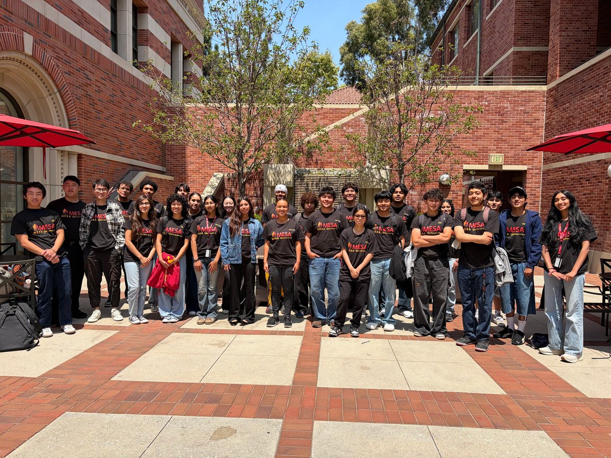
    🎉 Congrats to all the MESA MASTERMIND Summer Camp students! What a great way to kick off their STEM journey! Excited to see MathWorks and USC helping students get ready for what's ahead with #MATLAB!
    Download
    000
  5. MATLAB@MATLAB
    Think you can build your own fluid flow simulator? Here’s your shot. This interactive module lets you build one yourself—no PhD required. Try it, tweak it, break it. See what flows 👉 #CFD #MATLAB #FluidDynamics
    Download
    1291828.7K
  6. MATLAB@MATLAB
    📣 NEW MATLAB/Simulink Cheat Sheet 👇 Explore all the capabilities for Designing Feedback Control Systems while keeping them handy with this poster. Save this post or download it res here ➡️ #MATLAB #Simulink #MathWorks
    Download
    2211288K
  7. MATLAB@MATLAB
    Bring your plots to life! Animate with 4 techniques: 1️⃣ Update data in a loop 2️⃣ Matrix transformations (hgtransform) 3️⃣ Animated GIFs (exportgraphics) 4️⃣ Movies (getframe) 💡Tip: Always use drawnow in loops! #MATLAB #DataViz
    Download
    2242047.8K
  8. MATLAB@MATLAB
    🛑 STOP. You want this code! Inspired by Orion and Artemis I, check out this lunar mission trajectory simulation in #MATLAB and #Simulink. #LunarMission 🚀 Get the source code:
    Download
    12485
  9. Show more posts