#MathLab

Take a closer look. You’re seeing the thermal cycles of a modular multilevel converter (MMC), synchronized with its phase voltage waveforms. This 3D visualization from Simscape simulation data using an AI agent connected to MATLAB:

Future wireless networks like 6G will have to sense and understand the world around them. Learn more about how phased arrays enable integrated sensing and communication (ISAC) systems to communicate with and localize users:

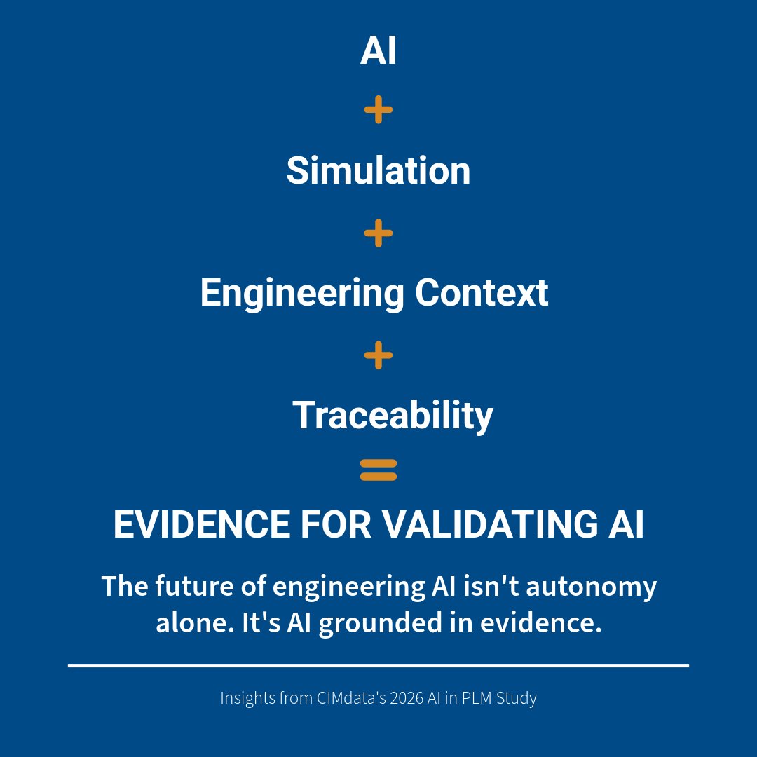
As AI agents take on more engineering tasks, how can teams trust the results? See how CIMdata examines validation, traceability, and evidence in AI-assisted engineering: Diego Tamburini takes the conversation further at MATLAB EXPO Online. #MATLABEXPO

TinyML Foundations and Applications on Arduino #Microcontrollers with #MATLAB 📕 Get Now:

🎃 Trick or treat? Credit to Vasilis Bellos for the original Mini Hack entry

Tomorrow! Join the global MATLAB and Simulink community at #MATLABEXPO Online. Explore AI, Agentic AI, Digital Engineering, Electrification, Robotics, and more. Registration is free, but required. Secure your spot today ⤵️

The Math Lab has only been opened for 12 days and we’ve already assisted close to 60 scholars! 🤓 Participants come from Algebra I to Calculus courses- all are welcome to join. #MathLab #LunchBunch @MsEstherRivera @ProvenzanoJohn

حل واجبات& رسالة ماجستير دكتوراه كتابة بحوث% قانونية لاب تصميم مواقع ويب مشاريع،،% إدارة الجودة تخطيط الموارد ERP مشروع تخرج÷، نظم المعلومات الإدارية MIS اسايمنت بروجكت في تحليل// تصميم الأنظمة تكليف هندسة البرمجيات Java برمجة C++ واجب_ MATLAB تطبيقات/ Excel المتقدمة

is for sale right now Get it before it goes in the vault 🏦 #math #mathlab #Maths #Mathematics #web3 #Nfts #nft #crypto #DeFi #Hive #ETH #Bitcoin #technology #business #venturecapital #sales #bigdata

Karman vortexのシミュレーションも瞬殺だぜ、MATLAB Codex

You don’t need a robotics degree to learn the math behind robots. University of Michigan has a 26-lecture course sitting on YouTube. Free. 🤖 It is the recorded lecture series from ROB 501, a graduate-level course covering much of the mathematical foundation used in robotics. Some of what it covers: → Abstract linear algebra → Linear operators & eigenvalues → Projection and least squares → Recursive least squares & Kalman filtering → Probability & Gaussian random vectors → QR factorization → Newton-Raphson → Real analysis & convergence → Linear programming These are not short overview videos either. Many of the lectures are around an hour long and work through the mathematics properly. The accompanying GitHub repository also includes the textbook, lecture notes, homework, exams, recitations, and MATLAB material. If you work in robotics, controls, estimation, perception, or ML and want stronger mathematical foundations, this is a very good resource to save. All 26 lectures are free.

🐍📰 MATLAB vs Python: Why and How to Make the Switch In this step-by-step tutorial, you'll learn about MATLAB vs Python, why you should switch from MATLAB to Python, the packages you'll need to make a smooth transition, and more. #python

Solving Partial Differential Equations using Physics-Informed Neural Net. A MATLAB Implementation. Let’s say we’re to solve a 2D wave equation 𝑢𝑥𝑥 + 𝑢𝑡𝑡= 𝑓(𝑥,𝑡) 0<𝑥<1 and 0<𝑡<1 Suppose the partial differential equation has been solved analytically with solution 𝑢(𝑥,𝑡) = 𝑠𝑖𝑛(π𝑥)𝑠𝑖𝑛(π𝑡) consequently 𝑓(𝑥,𝑡) =-2π² 𝑠𝑖𝑛(π𝑥) 𝑠𝑖𝑛(π𝑡) with homogeneous Dirichlet condition 𝑢(0,1)= 𝑢(1,𝑡)=𝑢(𝑥,0)=𝑢(𝑥,1)=0 ——————————— The MATLAB architecture will have: two input neurons 𝑥, 𝑡 3 hidden layers with 32 neurons each 𝑡𝑎𝑛ℎ as the activation function 1 output neuron 𝑢(𝑥, 𝑡) We’ll the following Matlab commands 1. dlnetwork : to rep neural net 2. dlarray : to manage differentiable data 3. dlgradient: to calculate derivatives 4. dlfeval : to evaluate custom function 5. adamupdate : to update trainable param We need interiors and boundary points Let just use 500 interior points and 500 points on each boundary edge %code clc; clear; close all; rng(1234); % Number of points Nf = 5000; Nb = 500; % Interior collocation points x_f = rand(1,Nf); t_f = rand(1,Nf); % Boundary points s = rand(1,Nb); % boundaries X_left = [zeros(1,Nb); s]; X_right = [ones(1,Nb); s]; % Bottom and top boundaries X_bottom = [s; zeros(1,Nb)]; X_top = [s; ones(1,Nb)] X_b = [X_left, X_right, X_bottom, X_top]; % dlarray data X_f = dlarray(single([x_f; t_f]),'CB'); X_b = dlarray(single(X_b),'CB') ———————- The ‘CB’ in the code means channel and batch dimension The input matrix has dimension 𝑥 ε R²⁰²⁵ ————————- Define the neural network %% code layers = [ featureInputLayer(2, ... Normalization="none", ... Name="input") fullyConnectedLayer(32,Name="fc1") tanhLayer(Name="tanh1") fullyConnectedLayer(32,Name="fc2") tanhLayer(Name="tanh2") fullyConnectedLayer(32,Name="fc3") tanhLayer(Name="tanh3") fullyConnectedLayer(1,Name="output") ]; net = dlnetwork(layers); ———— To now calculate the partial derivative, the network approximate 𝑢(𝑥, 𝑡) =𝑢ᶿ(𝑥, 𝑡) We need 𝑢 ₓₓ + 𝑢ₜₜ To calculate the derivatives, the 𝑑𝑙𝑔𝑟𝑎𝑑𝑖𝑒𝑛𝑡 allow us to differentiate the network Δ𝑢θ = [ 𝑢ₓ 𝑢ₜ] Δ 𝑢ₓ = [𝑢ₓₓ 𝑢ₓₜ] Δ 𝑢ₜ = [ 𝑢ₜₓ 𝑢ₜₜ] we only need first component of the first vector and second component of second vect %% code function [u,uxx,utt] =Derivatives(net,X) %prediction u = forward(net,X); % First deriv gradU = dlgradient(sum(u,"all"),X, ... EnableHigherDerivatives=true); ux = gradU(1,:); ut = gradU(2,:); % Second deriv gradUx = dlgradient(sum(ux,"all"),X, ... EnableHigherDerivatives=true); gradUt = dlgradient(sum(ut,"all"),X, ... EnableHigherDerivatives=true); uxx = gradUx(1,:); utt = gradUt(2,:); end In the function, dlgradient expects a scalar differential, since we have thousands of interior points, summing all the prediction allow us to calculate their derivative in one shot ————- Next we construct the loss function Recall that 𝑢ₓₓ + 𝑢ₜₜ = 𝑓(𝑥, 𝑡) The residual is Rᶿ =𝑢ᶿₓₓ- 𝑢ᶿₜₜ ₋ 𝑓(𝑥, 𝑡 ) Total loss = PDEₗₒₛₛ - Boundaryₗₒₛₛ % code function [loss,gradients,lossPDE,lossBC] = modelLoss(net,X_f,X_b) %network derivatives [u,uxx,utt] = calculateDerivatives(net,X_f); %coordinates x = X_f(1,:); t = X_f(2,:); % Force function f = -2*pi^2*sin(pi*x).*sin(pi*t); % PDE residual residual = uxx + utt - f; % Physics loss lossPDE = mean(residual.^2, "all"); % Boundary predictions uBoundary = forward(net,X_b); % Boundary loss lossBC = mean(uBoundary.^2,"all"); % Total loss loss = lossPDE + 10*lossBC; gradients = dlgradient(loss,net.Learnables); end The network learn by satisfying the differential equation and it's boundary cond. ———- Next is to minimize the loss function. I'll use Adam optimizer algorithm to update the training param

#JavaScript #Mathlab #reactjs #typescript #100DaysOfCode #coding #webdevelopment #maths #python #Biochem #science #Assignment #Homework #business #Essay #payfinals #Appdev #Histor #All maths code problem #Biotechnology #Chemistry #ICT related HMU @Olwriter50

レーシングカーはなぜ直線で上下にバウンドするのか？ 車高を下げるとダウンフォースが増加しますが、下げすぎると気流が剥離して車体が浮き上がります。 このポーパシング現象の物理メカニズムを、MATLAB Agentic Toolkitによる可視化で分かりやすく確認できます。

残り少なくなっちゃった 2026 年。今年中に新しいことを試したい、そんな方ピッタリの無料チュートリアルの一覧じゃないですか（宣伝） だいたい 2 時間程度で修了想定のものばかりなので、新しい領域の味見にどうぞ！

MATLABのオンライントレーニング、ふと見ると入門コースが２６個になっていましたね どんなものがあるか、書きだしてみました📝

5 days of #summerschool @AROMA_CFD @Sissaschool #mathLab. Thanks to All participants, #lecturers, #poster #presenters. @SiamSissa @AROMA_CFD @RBniCS @rozzagroup #argos #mathematicsarea #cfd #reducedordermodelling visit:

I deliver quality work #Project #mathlab #Essay due English #Paperpay #Casestudy quiz Onlineclasses #Python #Javascript #Philosophy #bookreview #Assignmentdue #Chemistry #100DaysOfCode #WomenWhoCode #NodeJS #Code #US #UAE #KUWAIT Dm @Owriter75

Hire us for; #mathlab #excel #Project #math #Essay due #English . #Paper pay #Case study #quiz #Do my homework #Online classes #Python #Javascript #Philosophy #book review #Assignment due #Chemistry #physics #WomenWhoCode #history #100DaysOfCode #NodeJS @Olwriter50

Tonight's #Mathlab #makeandtake was a success and I am incredibly proud of the families that attended and grateful for the help of @Leek_Kathy &amp; Mr. M. #everychild @LandrumMS @MrsGuerrero2014 @mrroymoore @_ramirezinsixth @mathwithkathlms